Shapley value in the context of machine learning

Motivation

A topic that is often overlooked or underestimated by engineers or researchers, related to the machine learning field, is the issue of model explainability, understood as the interpretability of the criteria by which the algorithm was guided when providing answers to a given problem. Understanding the “background” behind a given business process, which is often critical to a given organization, seems obvious, but is regularly underestimated. Of course, there are industries where the discussed aspect is well recognized and addressed. The flagship examples are banking models, where there are special regulations specifying requirements in this regard. The European Union responds to this need in its document “WHITE PAPER: On Artificial Intelligence – A European approach to excellence and trust”, where the need to interpret models is highlighted.

Having already outlined the bigger picture, we can move on to the methods that enable the aforementioned interpretation. One of them is the significance of the model features, i.e. the impact of a given column of data on the obtained results. Such information can explain a lot and lead to the next steps. Some algorithms, such as regression or decision tree, make it possible to extract the significance of particular features relatively easily. If we want to have a more universal technique, independent from the algorithm used and its implementation, we have to delve into the mathematics involved.

Shapley values

Shapley value (Shap-value) is a concept developed in game theory that has increasing interest among machine learning practitioners in the context of variable significance explanations in predictive models. Its primary use is to assess the impact of individual players on the outcome of a coalition game, while in machine learning it is used to assess the impact of individual variables on the predicted value.

However, there are claims that such borrowing of a concept from game theory is not necessarily appropriate in the context of the purpose of explaining the influence of variables on the model. A summary of this criticism is provided in the article “Problems with Shapley-value-based explanations as feature importance measures” by IE Kumar, S. Venkatasubramanian, C. Scheidegger, and SA Friedler. The authors raise both mathematical issues arising from the definition of Shapley’s value and the inconsistency with what we understand as an explanation of the model.

In this post, we present the theoretical definition of Shapley’s value, the definition of Shapley’s value in the context of explaining the predictive model, as well as the authors’ criticism of the concept introduced.

Definition

Imagine a game in which a group of players work together for mutual benefit. Denote the respective numbers of players from 1 to N. The set² of all players is then {1, …, N}, but we will denote subsets of this with U ⊆ {1, …, N}. For any subset U, one can define the value v(U) defining the benefit from cooperative game players in U. For example, v({1,…, N}) is the result of playing with all the players. We assume that v(∅) = 0. Intuitively, having a certain number of participants of a given game (say hide and seek) at our disposal, which we denote with N, we create different groups from them called U. Each group plays one game and then the game is assessed (for example, the level of satisfaction of the participants). The rating is marked as v.

The goal of Shap-value is to evaluate how much influence the individual players have on the outcome of the games. Let’s take a player with the number i. For any subset of U, we can define the influence of Player i on the improvement of the result.

Let’s try to understand the above notation better: imagine two groups of players differing in one player, called i. In order to assess its influence on the game, we will play two matches—one in the group with Player i and the other without Player i. The other participants remained the same. At the end of each game, an evaluation is made of v (U ∪ {i}) and v (U), respectively. Their difference is interpreted as the impact of Player i on the game. But is this an honest assessment? Not completely. This is due to the multitude of player combinations. A given player may be more useful in combination with certain players and less so with others. To reduce the risk of a possible mistake, we have to repeat the experiment for all possible combinations of players. Then the Shapley value for Player i is defined as the weighted average of all possible subsets of U.

More precisely, let Π be the set of all permutations of the sequence (1, …, N). Then, for any π ∈ Π the set

is the set of all players preceding Player i in the permutation π. We can then define the Shapley value as follows:

Where N! is the number of all permutations in Π, so the above value is just the arithmetic mean of all permutations.

The above notation is a mathematical representation of our previous intuitions. In this way, we get the Shapley value for Player i as the average value of the contribution (in the context of function v) that the player adds to each of the subsets of players (games).

Significance of variables

The above approach translates into the problem of determining the significance of variables in the predictive model. Let us take a model f that depends on many variables. In this situation, we will treat the variables as players from the previous definition. Let’s assume

where d is the number of columns in the set, x is the symbol of a single column, and X is the set of columns. Let’s look at the function v(U), evaluating the benefits of using the set U. What could such a function be in our case?

Example

Let us assume for a moment that we are using a linear model for a regression problem. One of the universal metrics for assessing the quality of the regression model is R2 (we previously assessed player satisfaction). Let us assume the value of R2 of the model trained on variables with U as v(U). Then, the partial influence of the variable i, defined earlier as

is the value by which R2 is improved after adding the i-th variable to the model based on U.

Example in Python

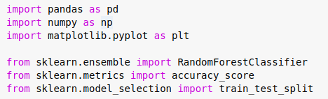
Let’s move away from thought experiments for a moment and work on the code. As an example, we will use the popular Irys Dataset collection. This is a classification problem where we try to predict a flower species based on a set of features. Therefore, the use of the R2 metric would be wrong. Let’s change to the popular accuracy metric. Before we start, let’s first prepare the environment and load the data.

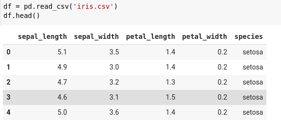
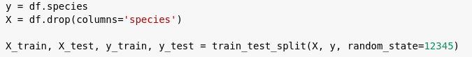
The data do not require any additional transformations. The number of rows is 150, while the number of classes (target) is 3. The next step is to divide the data into training and testing sets.

In the example, the already mentioned that the accuracy metric will be considered as a function v(U). For each subset, a model containing the tested feature and a model without this feature will be trained. Differences in accuracy values ​​will be recorded and averaged. Finally, the obtained results represent the average improvement in the accuracy of the model after adding the variable.

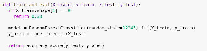
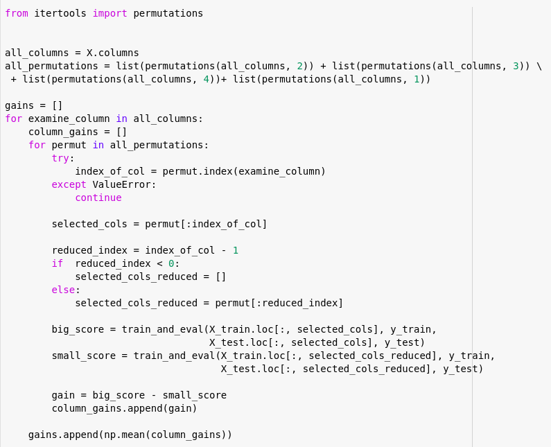
The careful reader will notice an assumption. It has been assumed that, for a model built on an empty set (without data), the prediction will be random, i.e. one of the three available classes will be selected with equal probability, hence the function train_and_eval returns the value 0.33 in certain cases. Let’s go to the results:

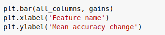
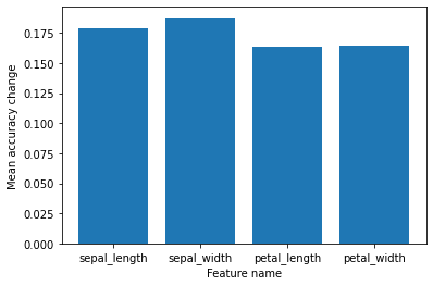
From the graph, we can conclude that getting rid of any of the available columns will not significantly affect the result. The small amount of data in the dataset used in the example may be problematic. Perhaps, with a larger set, the differences would be more pronounced.

Effect on the result. Locality.

The example above was just a simple representation of the function v. Let’s move on to the more popular approach. Think of Shapley value as an estimate—how much the feature i changes the prediction value of the model f(x).

Let us recall the expressions defining Shapley Value:

For Δv to be a “change in the prediction value” under the influence of a variable, v(U) and v(U ∪ {i}) should be the prediction values ​​on models trained only with variables U and U ∪ {i}, respectively. The problem with this approach is that we would then have to train a lot of models—2 to the power of d. Therefore, approximations of such “isolated” models are used, e.g. by averaging the values ​​of the full model, conditioning it on the variables from the set. Call it …

Let’s stop here for a moment and simplify things a bit. According to the definition, in order for our estimation to be as close to the truth as possible, we need to train a very large number of models. For example, for a set with 30 features (there are situations where we have thousands of columns at our disposal), we have 30!, so 2.6525286e + 32 possibilities. Training such a number of models is not feasible in a reasonable time (it would probably take a lifetime :)). Simplifications of the method are necessary to have any practical application. The one described here consists of the extraction of a part of the algorithm, where calculations do not take into account the considered feature. Thanks to this, it can be replaced with the average value, which significantly speeds up the computation time. Ending the intuitive digression, let’s return to the mathematical part.

… by the so-called conditional expected value

which is the average value of the model f(X) with variables from the set U, set as

These are the values ​​determined for specific xᵤ. In order to obtain v(U), the above values ​​should be averaged over all possible x; therefore, we assume the following notations:

In the above approach, it is not clear how to determine

in individual models. An effective way of determining such values ​​can be performed for tree algorithms. The method implemented in TreeSHAP algorithms uses the ability to quickly check the values ​​in the leaves into which the variables fall under the conditions.

The problem with unambiguity

The main problem in the below approach

are variables that are deterministically dependent on others. Two variables in the model that are equal (with probability 1) will obviously have the same Shapley value, but the mere fact of including or not including a duplicate variable affects the Shap values ​​for the other variables, which makes their interpretations very difficult. This means that duplicate columns can be highly problematic.

Let’s see it with an example. Let us take a model with the variables X₁, X₂, and a duplicate variable X₃, i.e. such that

From the basic properties of the conditional expectation value, we know that

Therefore

and

considering the same model only with two variables X₁ and X₂,

we get the following values:

We can see that, for both the first and the second variable, the values ​​are different in both models. There is also no simple relationship between ϕ′v (X₂) and values ϕv (X₂) and ϕv (X₃).

P.Adler proposed that dependent variables should be identified earlier and modelled with the rest of the variables.

Contrasting sentences

One of the issues raised is translating dependency/causation from contrastive sentences. How do you answer the questions “Why did P instead of Q happen?” or “Why should we consider variable i instead of throwing it away?” Some answer to this type of questions gives us the value

More precisely: Why add the variable i to the set U? Because it increases the value of v by Δv(i, U).

The problem with such an explanation arises when we take the mean over all U while calculating the Shape-value ϕv(i). Then we lose the information about the set to which we are adding, for which set this profit is the highest, for which set this profit is negative, or for which set the impact has the opposite sign compared to calculated mean.

For example, such information is better used in stepwise selection methods, where variables are successively added to the model based on the information that causes the greatest profit.

This is an important observation. Shap value is averaging over all possible groups, so it is natural to find a group of players for which a given feature has a completely different effect than it would appear from the Shapley value. For example, by adding variables to the model iteratively one at a time, it is better to calculate the profit only for the previously selected variables. By checking the pool of available variables in this way, we will be able to determine the optimal order of adding features to the model (feature ranking). Thanks to this, we obtain the possibility of balancing between the effectiveness of the model and its computational requirements.

Influencing the result

The second issue highlighted by the authors is explaining the possibility of influencing the model result. The Shap-value construction, unfortunately, does not allow us to unequivocally say how to change any of the variables to increase the model result, e.g. by 0.1, which can be said with simpler constructions, as in an ordinary linear regression model; the value of the coefficient standing at it tells us by how much the result will change if we increase the value of a given variable by 1.

Moreover, a positive Shap value does not always mean that increasing the value of the variable will increase the model’s score.

Python Usage Example

Let’s follow one more example of using Shap value in Python. This time I will use a package dedicated to this. For this purpose, I will use the decision tree model, trained on Irys Dataset—the same one that was used in the previous example. The steps involved in preparing the environment and loading the data are the same for both examples, so I will omit them. Let’s go straight to training the model.

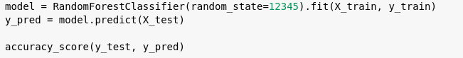
The result achieved by the model is 0.947 in the accuracy metric, which is very high.

The random forest model implemented in the sklearn package has a built-in ability to determine the most important features. Let’s see how it looks.

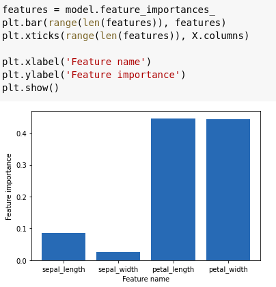
Features related to the size of the petal turn out to be decisive. Let’s verify if the results returned by the Shapley values ​​package match the previous observations.

Shapley values ​​in Python

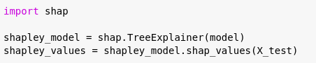
One of the available implementations of Shapley values ​​is the package shap. Ongoing code will be based on said module. The basic object we will work with is the TreeExplainer class. Basically, all the work is about calling the appropriate methods. Let’s start with .shap_values ​​(), which determines the Shapley values.

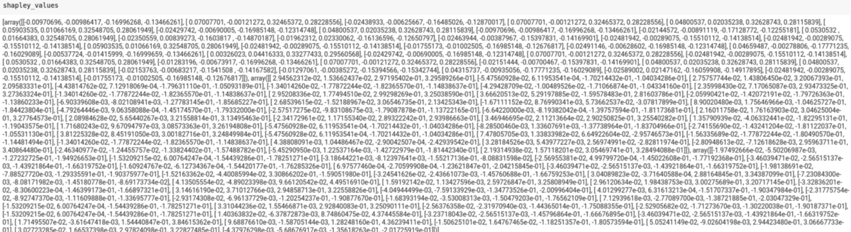
Is this the end? Basically yes, for the math part. Unfortunately, the results are completely messy. So far, we have a list of elements where each of them is a matrix in the format number_observations x number_features, showing the effect of the feature – observation combination on a given class. For this reason, our list has three items—one for each class, and each of them is 38×4 (test set only). Let’s look at the first matrix.

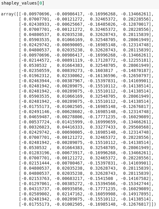
You can notice that the last two columns take larger values, but this is not well-readable information. How do we transform raw data from tables into a more human-friendly form? Fortunately, the authors of the pack thought about it.

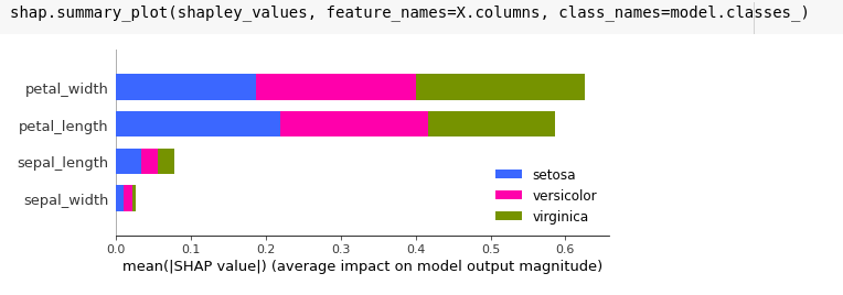
The method summary_plot allows you to make a quick and visually friendly summary of the importance of features for individual classes. Note a feature of this plot: all values ​​are positive. If we calculate the average values ​​for each class ourselves, we get a slightly different result…

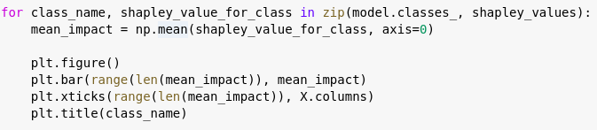
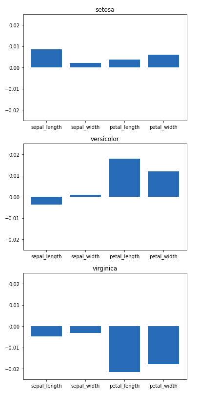
…but it results only from the form of data presentation, which may or may not include the sign of the value.

Note one more aspect that does not arise directly from the presented theory, namely the presentation of separate Shapley values sets for each class. In the case of classification models, the values ​​are calculated based on the score (in the case of the implementation available in the shap package)—the probability of belonging to a given class. In the case of the model operating on three classes, we have three scores corresponding to belonging to a given class. With this information at your disposal, it’s worth taking advantage of. This is what the discussed model does. However, there are cases where we are not interested in the impact of a given feature on a given class, but in its overall impact on the model. In these situations, the contributions of a given feature for all classes should be summed up, but without taking into account the sign (sum of absolute values). For a chart obtained from the method summary_plot, this will be the value of the bar outline.

Finally, one should mention another issue, namely the difference between the SHAP algorithm (SHapley Additive exPlanations)³ implemented in the shap package, and the basic Shapley value algorithm. The latter, as was described in the theoretical part, determines the average effect of the feature on the model. In our example, we estimated the mean increase of the accuracy metric for each feature. On the other hand, SHAP, instead of averaging, sums up the growth of the selected function v. This is the reason why the results obtained by means of the classic Shapley value and SHAP differ from each other. In practice, the latter is the much more common solution.

To sum up, Shapley values ​​seem to be an interesting tool to better understand our model. They can also be used in the process of selecting features as an indicator of their suitability. The results obtained with the package shap are consistent with the mechanism built into the sklearn model feature_importance.

¹ https://en.wikipedia.org/wiki/Shapley_value

² as a reminder, sets in mathematics are marked with curly brackets {}. A set is a collection of any entity, especially numbers.

³ Lundberg, Scott M., and Su-In Lee, “A unified approach to interpreting model predictions.” Advances in Neural Information Processing Systems, 2017.

⁴ https://christophm.github.io/interpretable-ml-book/shap.html